-
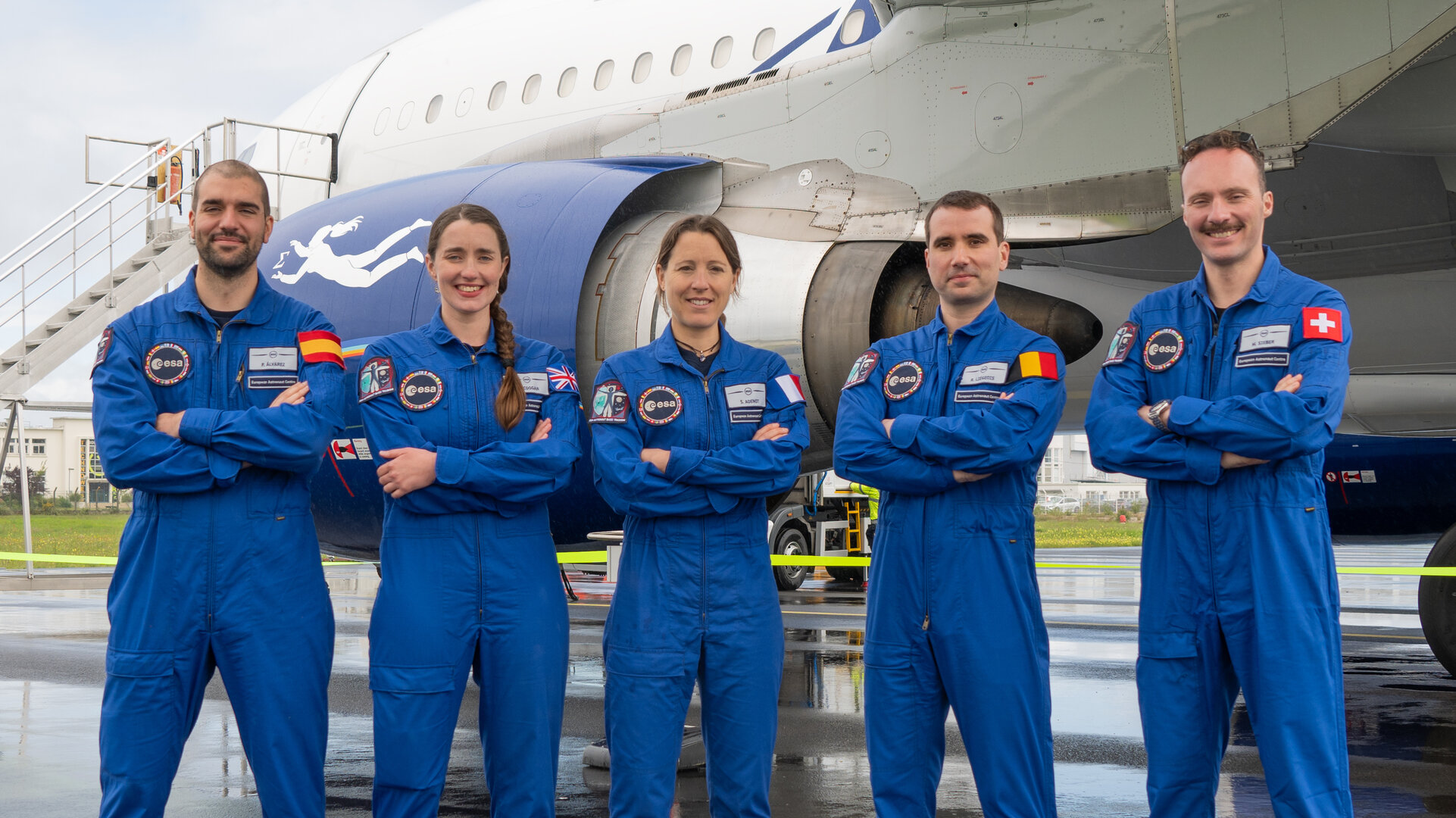
VideoScience & Exploration
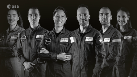
ESA astronaut class of 2022 graduation ceremony replay

-
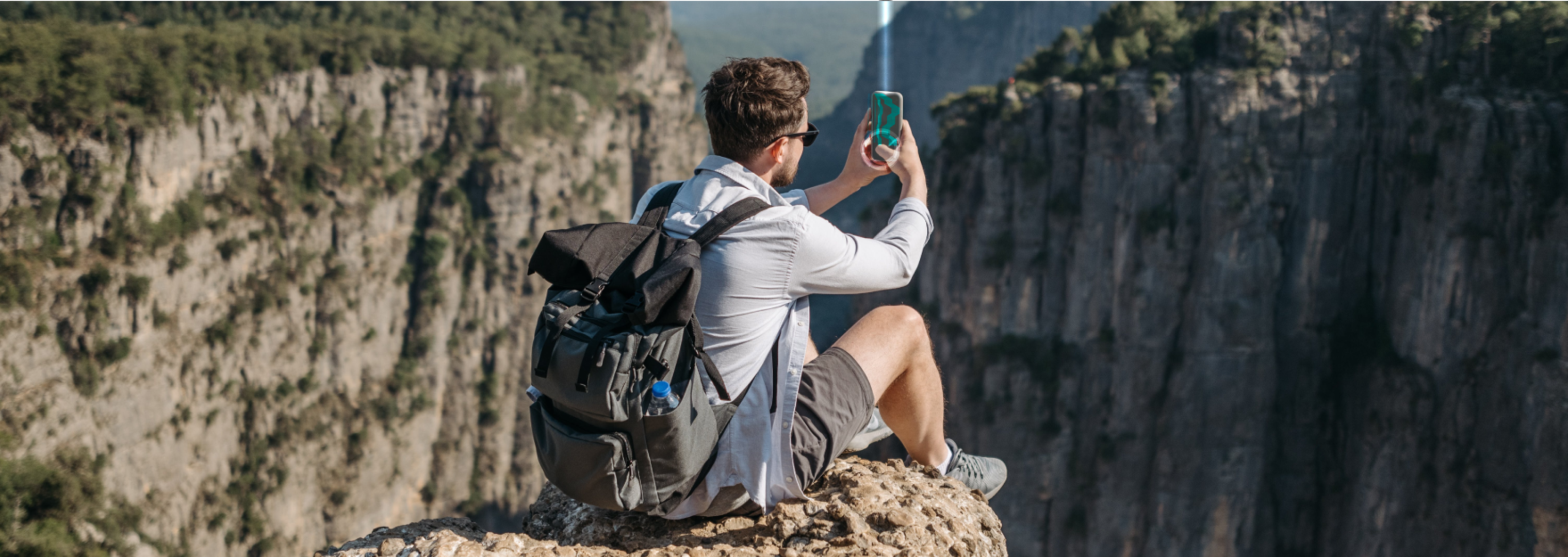
StoryApplications
Six mind-blowing facts about Galileo
-
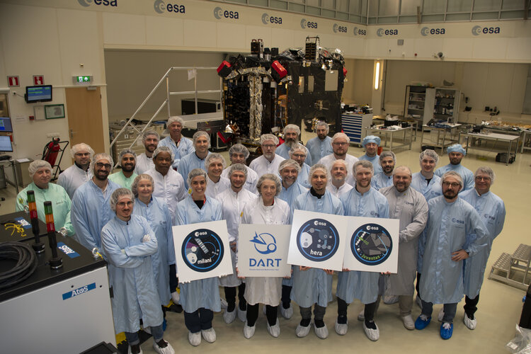
VideoSpace Safety
The Incredible Adventures of the Hera mission – The Missing Puzzle Piece

-
StoryAgency
Discover ESA Live: a gateway to ESA’s universe for schools

ESA Programmes
ESA and You
In the spotlight


Image
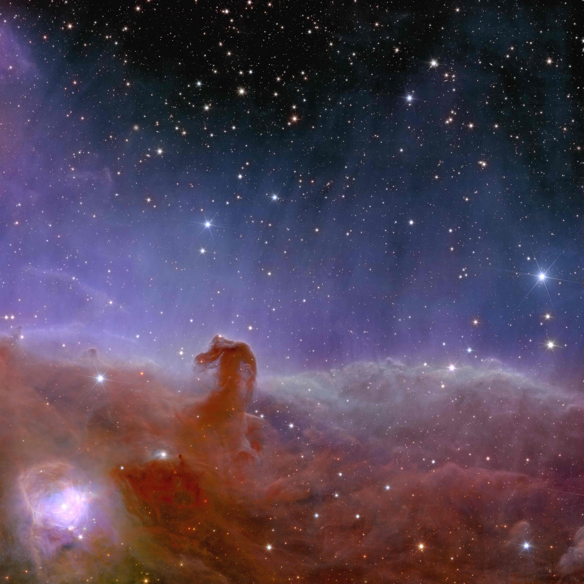
Science & Exploration
Euclid’s view of the Horsehead Nebula
Recommended


Image
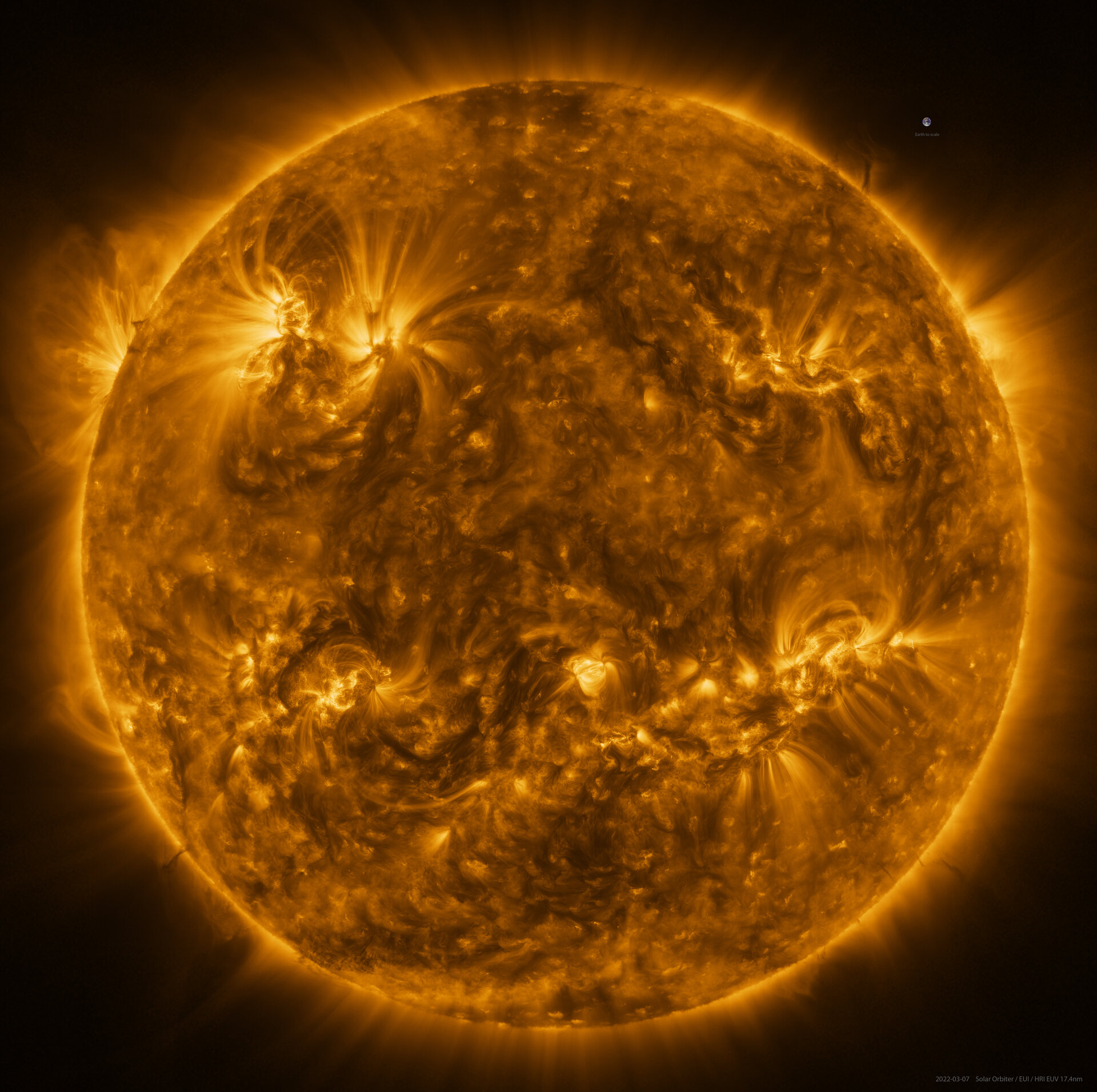
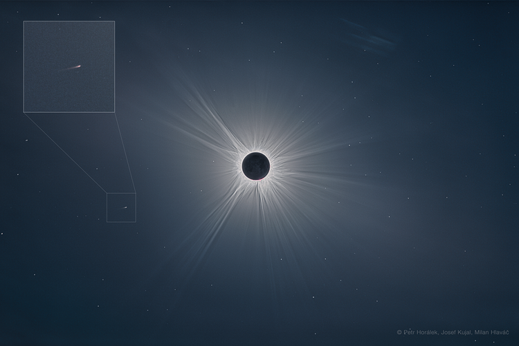
Science & Exploration
The Sun in high resolution