| | Urbanisation – Detection by means of delineation of the city perimeter
Page 12 12
This exercise is divided into two parts and requires the use of LEOWorks.
Part 1
After the visual evaluation and interpretation of these two high-resolution satellite images, you will carry on with the analysis of the urbanisation of Lhasa, and quantify the increase of urban area within the period from 1965 to 2000.
Download the necessary data from Himalayas_env3.zip.
As a first step, we will examine the two multispectral images of 1 Nov 1988 and 28 Dec 2000. Launch LEOWorks and open the following images: 1988_321.tif, 1988_432.tif, 1988_543, and 1988_753.tif.
1988_321 means: image of the year 1988 in natural colour, band 3 in Red, band 2 in Green and band 1 in Blue. 1988_432 has band 4, the near infrared, in Red, etc. Band 5 is infrared (around 1.6 μm), and band 7 is also infrared (around 2.2 μm)
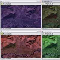
When you open the images, your viewer should look like this:
Different band combinations of 'Lhasa 1988'
As you can see, there is not a lot of contrast in the images, and it is hard to distinguish between the different types of land cover. This is because the grey values of the pixels in the images are quite close to each other.
Press the 'Image histogram' button in your viewer.
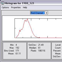
A window will open which shows the image histogram.
The histogram is presented for every channel of the image. As you know, colour images usually consist of 3 screen channels: a red, a green, and a blue screen channel.
The histogram below describes the distribution of the pixel- (or grey-) values for this channel.
As this is an 8-bit dataset, the image grey values can have a range between 0-255. This makes 256 different possible values for a pixel. 2^8 (2*2*2*2*2*2*2*2 = 256).
As you can see from the histogram, the majority of the grey values is between 9 and 128. When you move your mouse above the histogram, a crosshair appears and shows you, in the information box below, the value (level) and the count of total pixel with this specific value (count).
Only 119 (128-9) of the spectrum of 256 different grey values is used. As it is quite difficult for the human eye to distinguish colours that are quite similar, we can spread the information over the full spectrum of 256 possibilities.
Image histogram
In LEOWorks, press Enhance>Histogram Equalization. You can see the effect immediately after pressing the button. Go again to inspect the histogram after the equalisation. You willsee that the full spectrum is now used, and that contrasts in the image are represented in a much better way.
Do this step with all four images and compare them with each other.
1. Why does a digital image consist of 3 screen channels? What spectral bands might be behind (see the three examples)?
2. What would an optimal histogram look like?
3. Why did the original image not show any contrast and colours?
4. How do these 3 band combinations vary from each other?
5. What colour does vegetation have in these images?
6. What colour does urbanised areas have in these images? (Use the 'lhasa_1965' and 'lhasa_2000_3m' to distinguish the urban area from the farmland etc.)
After examining all the different images, which all show a different band combination, you will see that the objects appear in a different colour.
The different colours in these images derive from the different band combinations of the sensor. This image was taken on 1 November 1988 by the Landsat Thematic Mapper. It has a spatial resolution of 28.5 metres and 7 different bands (6 spectral, 1 thermal).
The spectral bands are described as follows:
Band 1: Blue
Band 2: Green
Band 3: Red
Band 4: Near-infrared
Band 5: Mid-infrared
Band 6: Thermal (not available here)
Band 7: Mid-Infrared
Page12
| |